If you are an NLP person, chances are you know PCFGs (probabilistic context-free grammars) pretty well. These are just generative models for generating phrase-structure trees.
A CFG includes a set of nonterminals (\(N\)) with a designed start symbol \(\mathrm{S} \in N\), a set of terminal words (the “words”) and a set of context-free rules such as \(\mathrm{S \rightarrow NP\, VP}\) or \(\mathrm{NP \rightarrow DET\, NN}\), or \(\mathrm{NN \rightarrow\, dog}\). The left handside of a rule is a nonterminal, and the right handside is a string over the union of the nonterminals and the vocabulary.
A PCFG simply associates each rule with a weight, such that the sum of all weights for all rules with the same nonterminal on the left hand-side is 1. The weights, naturally, need to be positive.
Now, a PCFG defines a generative process for generating a phrase-structure tree which is followed by starting with the starting symbol \(\mathrm{S}\), and then repeatedly expanding the partially-rewritten tree until the yield of the tree contains only terminals.
Here is an example of a phrase-structure tree, which could be generated using a PCFG:
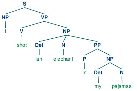
A phrase-structure tree taken from NLTK’s guide (http://www.nltk.org/book/ch08.html).
Each node (or its symbol, to be more precise) in this tree and its immediate children correspond to a context-free rule. The tree could have been generated probabilistically by starting with the root symbol, and then recursively expanding each node, each time probabilistically selecting a rule from the list of rules with the left handside being the symbol of the node being expanded. I am being succinct here on purpose, since I am assuming most of you know PCFGs to some extent. If not, then just searching for “probabilistic context-free grammars” will yield many results which are useful to learn the basics about PCFGs. (Here is a place to start, taken from Michael Collins’ notes.)
What is the end result, and what is the probability distribution that a PCFG induces? This is where we have to be careful. First, a PCFG defines a measure over phrase-structure trees. The measure of a tree is just the product of all rules that appear in that tree \(t\), so that:
$$\mu(t) = \prod_{r \in t} p_r.$$
Here, \(r \in t\) denotes that the rule \( r\) appears in \(t \) somewhere. \( t \) is treated as a list of rules (not a set! a rule could appear several times in \( t \), so we slightly abuse the \( \in \) notation). \( p_r \) is the rule probability associated with rule \( r \).
You might be wondering why I am using the word “measure,” instead of just saying that the above equation defines a distribution over trees. After all, aren’t we used to assuming that the probability of a tree is just the product of all rule probabilities that appear in the tree?
And that’s where the catch is. In order for the product of all rule probabilities to be justifiably called “a probability distribution”, it has to sum to 1 over all possible trees. But that’s not necessarily the case for any assignment of rule probabilities, even if they sum to 1 and are positive. The sum of all measures of finite trees could sum to *less* than 1, simply because some probability “leaks” to infinite trees.
Take for example the simple grammar with rules \(\mathrm{S \rightarrow S\, S}\) and \( \mathrm{S \rightarrow a} \). If the rule probability \(\mathrm{S \rightarrow S\, S}\) is larger than 0.5, then if we start generating a tree using this PCFG, there is a non-zero probability that we will never stop generating that tree! The rule \(\mathrm{S \rightarrow S\, S}\) has such large probability, that the tree we generate in a step-by-step derivation through the PCFG may potentially grow too fast and the derivation will never terminate.
Fortunately, we know that in a frequentist setting, if we estimate a PCFG using frequency count (with trees being observed) or EM (when trees are not being observed, but only strings are being observed), the resulting measure we get is actually a probability distribution. This means that this kind of estimation always leads to a *tight* PCFG. That’s the term used to denote a PCFG for which the sum of measures over finite trees is 1.
So where is the issue? The issue starts when we do not follow a vanilla maximum likelihood estimation. If we reguarlize, or if we smooth the estimated parameters or do something similar to that, we may end up with a non-tight PCFG.
This is especially true in the Bayesian setting, where typically we put a Dirichlet prior on each of the set of probabilities associated with a single non-terminal on the left handside. The support of the Dirichlet prior is all possible probability distributions over the \(K\) rules for nonterminal \(A\), and therefore, it assigns a non-zero probability to non-tight grammars.
What can we do to handle this issue? This is where we identified the following three alternatives (the paper can be found here).
- Just ignore the problem. That means that you let the Bayesian prior, say a factorized Dirichlet, have non-zero probability on non-tight grammars. This is what people have done until now, perhaps without realizing that non-tight grammars are considered as well.
- Re-normalize the prior. Here, we take any prior that we start with (such as a Dirichlet), remove all the non-tight grammars, and re-normalize to get back a probability distribution over all possible tight grammars (and only the tight grammars).
- Re-normalize the likelihood. It has been shown that any non-tight PCFG can be converted to a tight PCFG which induces a distribution over finite trees which is identical to the distribution that we would get from the non-tight PCFG, after re-normalizing the non-tight PCFG to become a distribution over the finite trees by dividing the probability of all finite trees by the total probability mass that the finite trees get (Chi, 1999). So, one can basically map all non-tight distributions in the prior to tight PCFG distributions according to Chi’s procedure.
Notice the difference between 2 and 3, in where we “do the re-normalization.” In 2, we completely ignore all non-tight grammars, and assign them probability 0. In 3, we map any non-tight point to a tight point according to the procedure described in Chi (1999).
The three alternatives 1, 2 and 3 are not mathematically equivalent, as is shown in this Mathematica log. But we do believe they are equivalent in the following sense: any prior which is defined using one of the approaches can be transformed into a different prior that can be used with one of the other approaches and both would yield the same posterior over trees, conditioned on a string and marginalizing out the parameters. That’s an open problem, so you are more than welcome sending us ideas!
But the real question is, why would we want to handle non-tight grammars? Do we really care? This might be more of a matter of aesthetics, as we show in the paper, empirically speaking. Still, it is worth pointing out this issue, especially since people have worked hard to show what happens with non-tightness in the non-Bayesian setting. In the Bayesian setting, this problem has been completely swept under the rug until now!
Notes:
- 1. For those of you who are less knowledgable about Bayesian statisitics, here is an excellent blog post about it from Bob Carpenter.
- Non-tight PCFGs are also referred to as “inconsistent PCFGs.”